Introduction
Amazon Forecast is a fully managed service that uses machine learning to deliver highly accurate forecasts, based on the same technology used at Amazon.com. Announced at re:Invent 2018 and Generally Available in August 2019, it was especially exciting to see how this service could be applied to solve problems that our eCommerce and Contact Center customers encounter around inventory and agent demand forecasting respectively.
Especially compelling is that Amazon Forecast has a few predefined Dataset Domains and Types, which allowed us to build our test scenario with relative ease. In addition to the Dataset Domain we are using for our test scenario, WORK_FORCE, there also exists domains for RETAIL, INVENTORY_PLANNING, EC2 CAPACITY, WEB TRAFFIC, METRICS and a CUSTOM domain for which a pre-defined domain does not exist.
Getting Started
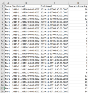
As far as the workflow goes, you start creating a dataset import (Dataset group > Dataset Name > TARGET_TIME_SERIES > Dataset import > s3 Bucket(s)) which is a CSV formatted file available in an S3 bucket that contains your time-series data. In our test case this would be the Queue-based Historical Metrics Report, containing “Contacts Handled Incoming” field, grouped by queue and then interval (30 minute). This provides us with the actual demand of a given queue (type) at a frequency of every 30 minutes, or 48 intervals a day. While Amazon Forecast is capable of accepting a variety of frequencies, the key to a reliable outcome is selecting the frequency appropriate to the source of data – infrequent data should use longer frequencies, as an example.
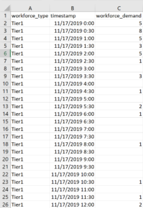
Since the Amazon Connect report only contains the previous 3 days of data at the 30 minute interval level of granularity and for our dataset we will want to start with 7 days of data to account for a typical call volume week, we will need to run the report three times throughout the week and join the data together in a single CSV, removing the EndInterval column and reformatting the StartInterval column to use a space instead of a T and remove the Z altogether, so your timestamp goes from yyyy-mm-ddThh:mm:ss.mmmZ to yyyy-mm-dd hh:mm:ss.mmm. You will also want to rename the columns to match that of your data schema. Queue becomes workforce_type, StartInterval becomes timestamp and Contacts Handled Incoming becomes workforce_demand. Following these steps you can use the Amazon Forecast import timeseries data wizard defaults and only need to select your data interval, which is 30 minutes. In the end you will end up with something like this:
After your import completes (a few minutes, based on the size of your data), you can find a summary of the job and any errors encountered during the import:
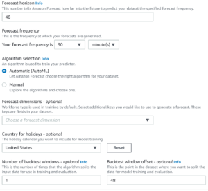
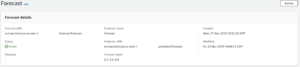
As this import was successful you can now move on to creating a predictor. In this wizard we define how far into the future we want to be able to forecast, or predict, based on the data in the imported dataset.
The maximum value we can set for the forecast horizon must be less than or equal to the maximum value of the backtest window offset (which can be up to 1/3 of the total number of frequencies in the imported dataset).
Since our dataset is rather small, we will start by setting the value of both to 48, which, being our frequency of data is every 30 minutes allows us to predict 1 day into the future. Moving on we will set the forecast frequency to be 30 minutes and let Amazon Forecast determine the best algorithm for our needs (AutoML), set an (optional) country to evaluate a holiday calendar against, and finally a backtest window offset to use for model training and evaluation:
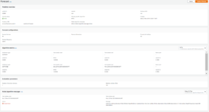
After the predictor execution completes (around 30 minutes for 3 days of 30 minute interval data, around 60 minutes for 7 days of 30 minute interval data) you can evaluate the results of the predictor execution, and in the case of AutoML, see the winning algorithm:
With a predictor created and an algorithm successfully selected you can move on to creating a forecast with the predictor you just created along with the quantiles you wish to forecast (.01 to .99 as well as mean, up to 5 can be selected):
Finally, with the forecast created we can now generate an export of our forecasted intervals as a CSV in an S3 bucket or interact with them in the console using Forecast lookup:
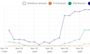
Here we can see our P50 forecast tracks closely to the actual demand:
Conclusion:
Amazon Forecast brings machine learning powered predictive forecasting to developers and power users without requiring heavy experience in data science or machine learning. A number of out of the box domains provides an easy path to get started for users in a variety of applications.
A clear benefit identified during the execution of this test case is the ease at which we can use Amazon Forecast to experiment – different configurations and combinations of datasets, predictors and forecasts can be run concurrently to identify the ideal configuration for our test case, without needing to wait for one to finish before starting the other.
Further, getting started with Amazon Forecast is easy – most of the actions are Wizard driven through the console, there is a multitude of documentation available at https://aws.amazon.com/forecast/ as well as usable examples available at https://github.com/aws-samples/amazon-forecast-samples. The samples are especially beneficial to new users as they contain a CloudFormation template to create a Sagemaker Notebook Instance that has a series of Jupyter notebooks available, containing well-defined sample data sources, walking you through the steps you would need to take to perform your first forecast.
Next Steps:
Taking this test case further, we can automate the export of the Amazon Connect Historical Report on a daily basis, writing it to S3. An S3 event can start a Lambda function to process the file, preparing it to be imported into Amazon Forecast. Once the Lambda function has processed the file, the Amazon Forecast Dataset Import job can be started, followed by a new Predictor Job and finally a Forecast Job. Once the Forecast job has completed the forecast can be exported to S3 to populate a datalake, crawled with Glue and visualized/reported on with QuickSight.


